8 Representation Learning
Every predictive model is really two models stacked together: something that turns raw input into a useful internal description, and something that turns that description into an answer. Classical machine learning put all the effort into the second half and left the first half to humans — a practitioner would hand-engineer features (pixel histograms, n-gram counts, ratios and interactions between raw columns) and feed them to a comparatively simple model. Representation learning is the bet that the first half can be learned too: instead of hand-designing what a “useful” description of the data looks like, train a model to discover one, using the data itself as the teacher.
This bet turned out to be the single biggest lever in modern AI. A learned representation that captures the task-relevant structure of the data — that places semantically similar things near each other, that discards nuisance variation like lighting or phrasing, that exposes the axes along which the data actually varies — makes every downstream problem easier, sometimes trivially easier. A linear classifier on top of a good image embedding can outperform a hand-engineered pipeline from a decade earlier; a nearest-neighbor search over sentence embeddings can do semantic retrieval that keyword matching structurally cannot. The central question of this chapter is not whether learned representations help — it’s how you get a model to produce them, and what kind of structure it ends up capturing depending on how you ask.
8.1 How it works
At the most basic level, a representation is just a map \(z = f(x)\) from raw input \(x\) into some other space, usually lower-dimensional or more structured, where \(z\) is easier to work with than \(x\) was. The question is what objective forces \(f\) to discover a useful map rather than an arbitrary one. Three broad answers dominate: reconstruct the input from a compressed version of it (autoencoding), predict something else about the data from a masked or contextual view of it (self-supervised prediction), and pull related examples together while pushing unrelated ones apart (contrastive learning). All three share a property worth naming explicitly: none of them need labels. They extract structure from the data’s own internal consistency, which is exactly what makes them scalable — you can run them over far more data than you could ever afford to label.
Classical foundations: linear representation learning first
Before neural representation learning, there was linear representation learning, and it’s worth understanding why it works before seeing where it breaks.
PCA finds the directions of maximum variance in the data. Formally, given centered data \(X \in \mathbb{R}^{n \times d}\), PCA finds an orthogonal projection to \(k\) dimensions that maximizes the variance of the projected data — equivalently, the projection that minimizes reconstruction error under a linear decoder. Both views are the same optimization: the top \(k\) eigenvectors of the data covariance matrix \(\frac{1}{n} X^\top X\) (or equivalently the top \(k\) right singular vectors of \(X\)) span the subspace that both captures the most variance and reconstructs \(X\) best in a squared-error sense. This equivalence — a linear autoencoder with a linear decoder and squared reconstruction loss recovers exactly the PCA subspace — is the conceptual bridge into the next section: an autoencoder is what you get when you replace PCA’s linear encoder and decoder with nonlinear ones.
Matrix factorization applies the same idea to structured interaction data. Given a user-item matrix \(R\) (ratings, clicks, purchases), it factors \(R \approx U V^\top\) where \(U\) and \(V\) are low-rank matrices of latent user and item factors. This is PCA’s sibling for sparse, incomplete data — it’s covered in depth in Information Retrieval, Ranking, and Recommenders, but it belongs here too, because it’s a canonical case of representation learning discovering latent structure (taste dimensions, genre affinities) that was never explicitly labeled.
Word2vec-style embeddings learn representations from co-occurrence: a word’s vector is trained so that it predicts (or is predicted by) the words around it in context. This is the first widely successful instance of the self-supervised idea that now underlies almost everything in Deep Learning Foundations and Generative AI and Foundation Models: you don’t need human labels if the data has enough internal predictive structure to generate its own supervision signal (predict the next word, predict the missing word, predict the surrounding context).
Autoencoders and why nonlinearity matters
An autoencoder generalizes the PCA picture with two neural networks — an encoder \(f_\theta(x) = z\) that compresses input into a latent code, and a decoder \(g_\phi(z) = \hat x\) that reconstructs the input from that code — trained jointly to minimize reconstruction error, typically \(\| x - \hat x \|^2\). Because the encoder and decoder can be arbitrary nonlinear functions (multi-layer networks with nonlinear activations), the bottleneck can learn curved, folded manifolds that no linear projection can represent.
Figure 8.1 makes this concrete. A Swiss roll — a 2D sheet curled into a spiral in 3D space — is a synthetic but honest stand-in for the kind of nonlinear manifold structure real data often has (think of a face rotating in 3D, or a robot arm’s joint-angle space). PCA, being a linear projection, can only ever produce a shadow of the roll: it flattens the 3D coordinates onto their two directions of greatest variance, which cuts straight through the spiral and leaves points from different “layers” of the roll tangled together in the 2D projection. A small nonlinear autoencoder (a 3 → 8 → 2 → 8 → 3 network with tanh activations, trained by plain gradient descent on reconstruction error) instead learns to route the data through its 2-unit bottleneck in a way that respects the manifold’s actual geometry more closely, because nothing constrains it to a single global linear direction — it can bend.
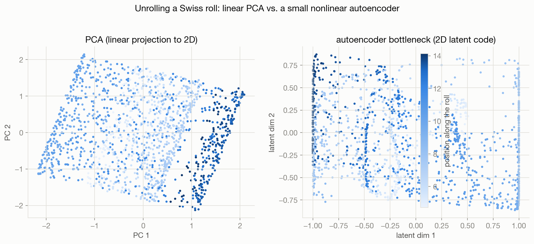
The comparison also illustrates the honest cost side of the tradeoff: the autoencoder needed an iterative nonconvex optimization (gradient descent with all its usual sensitivities — initialization, learning rate, number of epochs) to reach even this result, whereas PCA is a single closed-form eigendecomposition with no hyperparameters and a global optimum guaranteed. Nonlinearity buys expressiveness at the cost of optimization difficulty and interpretability — you can no longer point at a “latent dimension” and say precisely what linear combination of inputs it corresponds to.
8.2 Main methods
Denoising and sparse autoencoders
A plain autoencoder with a bottleneck narrower than the input is forced to compress, but if the bottleneck is not narrower — or if the model is powerful enough — it can cheat by learning something close to the identity function, which reconstructs perfectly but represents nothing useful. Two classical fixes constrain the model differently. A denoising autoencoder corrupts the input (adds noise, masks pixels or tokens) and trains the model to reconstruct the clean original from the corrupted version — this forces the representation to capture the underlying structure of the data rather than memorizing an identity map, since identity mapping the corrupted input would reconstruct the corruption, not the original. A sparse autoencoder instead keeps the bottleneck wide but penalizes the number of active latent units, encouraging each input to be explained by only a small subset of learned features — this tends to produce more interpretable, disentangled factors, and the same sparsity idea resurfaces today in mechanistic interpretability work that trains sparse autoencoders on top of large language model activations to find human-interpretable “features.”
Variational autoencoders
A VAE turns the autoencoder into a proper probabilistic latent-variable model: instead of the encoder outputting a single latent vector, it outputs the parameters of a distribution (typically a mean and variance for a Gaussian) over the latent variable, and the decoder defines a generative model \(p(x \mid z)\). Training maximizes the evidence lower bound (ELBO) introduced in Sampling and Approximate Inference — reconstruction quality traded against how close the encoder’s distribution is to a simple prior (usually a standard Gaussian) via a KL-divergence penalty. The KL term is what makes a VAE more than an autoencoder with extra steps: it regularizes the latent space to be smooth and generatively usable — you can sample a random \(z\) from the prior and decode it into a plausible new example, something a plain autoencoder’s latent space, with no constraint on its shape, generally cannot support reliably. The mechanism that makes this trainable end-to-end is the reparameterization trick: instead of sampling \(z \sim \mathcal{N}(\mu_\theta(x), \sigma_\theta(x)^2)\) directly (a non-differentiable operation, since you can’t backpropagate through a random sampling step), you sample \(\epsilon \sim \mathcal{N}(0, 1)\) independently and compute \(z = \mu_\theta(x) + \sigma_\theta(x) \cdot \epsilon\) — this moves all the randomness into \(\epsilon\), which doesn’t depend on the parameters, so gradients can flow through \(\mu_\theta\) and \(\sigma_\theta\) via ordinary backpropagation.
Contrastive learning
Contrastive methods learn representations without any reconstruction at all. Instead, they define which pairs of examples should be considered “related” (two augmented crops of the same image, an anchor sentence and its true next sentence, a query and its correct document) and train the encoder so that related pairs land close together in representation space while unrelated pairs land far apart — typically via a loss like InfoNCE, which treats it as a classification problem: given an anchor and a batch of candidates, correctly pick out the true positive among many negatives. This sidesteps the whole reconstruction question (there’s no decoder, no pixel- or token-level loss to get right) and tends to produce representations that are excellent for downstream retrieval and classification, because the objective directly optimizes for what those downstream tasks need: distances in the representation space that reflect semantic similarity. This is the mechanism behind modern embedding models used for dense retrieval and behind image-text models like CLIP that align two different modalities into a shared space by treating matched image-caption pairs as positives.
8.3 When to use it / what can go wrong
PCA versus a neural encoder is the first fork. Reach for PCA (or its close relatives, like truncated SVD) when you need something fast, deterministic, and interpretable, when your data’s structure is plausibly close to linear, or when you have too little data to safely train a nonlinear model — PCA has no risk of overfitting the way an undertrained neural encoder can. Reach for a learned nonlinear encoder when the data has structure a linear projection cannot express (curved manifolds, discrete symbolic structure, cross-modal alignment) and you have enough data and compute to train it properly. As Figure 8.1 shows, the nonlinear model is not automatically better — it has more failure modes (bad initialization, insufficient training, an ill-chosen bottleneck width) and needs real care to actually pay off.
Bottleneck size is a real modeling decision, not a hyperparameter to set and forget. Too narrow, and the model cannot represent the data’s true degrees of freedom, so it discards information the downstream task needs; too wide, and — absent another constraint like denoising, sparsity, or a VAE’s KL penalty — the model has no pressure to compress at all and can degenerate toward memorization.
A VAE’s latent space is only as smooth and disentangled as the KL term lets it be, and there’s a genuine tension baked into the objective: pushing the KL term harder makes the latent space more regular and better for sampling, but trades off against reconstruction fidelity (this tension is explicit in the beta-VAE family, which reweights the KL term to trade one against the other deliberately). If reconstructions look blurry or generated samples look generic, that’s often the KL term winning too much of this tradeoff.
Contrastive learning is extremely sensitive to how negatives are chosen. Too-easy negatives (obviously unrelated examples) teach the model little; near-duplicate false negatives (things labeled “unrelated” that are actually similar) actively corrupt the learned geometry. Batch size and negative sampling strategy matter more for contrastive methods than for most other representation-learning approaches, because the loss is defined relative to whatever negatives happen to be in the batch.
Representations trained for one objective don’t automatically transfer to another. An embedding optimized for reconstruction is not necessarily good for classification; an embedding optimized for one modality’s contrastive task is not automatically aligned with another modality unless that alignment was explicitly part of training. Always validate a learned representation against the actual downstream task it will be used for, rather than trusting reconstruction loss or contrastive accuracy as a proxy for “will this embedding help my real problem.”
8.4 How this connects
- Sampling and Approximate Inference supplies the ELBO and the reparameterization trick that make VAEs trainable — a VAE is best understood as variational inference where the approximate posterior is amortized through a neural encoder.
- Deep Learning Foundations covers the architectures (MLPs, CNNs, transformers) and optimization machinery (backpropagation, gradient descent variants) that every neural encoder and decoder in this chapter is built from.
- Graphical Models and Latent Variables frames PCA, matrix factorization, and VAEs as members of one family: latent-variable models that explain observed data through hidden factors, differing mainly in whether the mapping between latent and observed space is linear (PCA, matrix factorization) or learned and nonlinear (VAEs).
- Information Retrieval, Ranking, and Recommenders is where contrastive and embedding-based representations do their most visible production work — dense retrieval and two-tower recommenders are representation learning applied directly to search and personalization.
- Generative AI and Foundation Models builds on this chapter twice over: VAEs are one of its core generative families, and the self-supervised, label-free training philosophy introduced here (predict masked or contextual structure instead of using human labels) is exactly what makes pretraining large foundation models possible.