17 Causal Inference and Experimentation
Most of this book is about prediction: given \(X\), estimate \(P(Y \mid X)\) or a point estimate of \(Y\). Causal inference asks a different question — given \(X\), what would \(Y\) become if we intervened and set some part of \(X\) ourselves? “Will this user churn” is a prediction question. “Will sending this user a discount stop them from churning” is a causal question, and a model trained to answer the first does not automatically answer the second, no matter how accurate its predictions are. This gap — between a model that explains the data as it naturally occurred and a model that tells you what happens when you change something — is the entire subject of this chapter. It matters everywhere a system makes a decision meant to change an outcome: pricing, ranking interventions, product experiments, medical treatment, policy, and increasingly, the actions an autonomous agent takes on a user’s behalf.
The reason the gap exists is confounding. In observational data, the variable a model would like to treat as a “cause” is usually entangled with other variables that independently affect the outcome and that also affect whether the “cause” occurs in the first place. A model fit to \(P(Y \mid X)\) happily learns these entangled associations because, for prediction, that’s correct and sufficient — a proxy is exactly as useful as the real thing if the world doesn’t change. The moment you act on the model’s output, you change the very statistical relationships it learned from, and the proxy breaks. Causal inference is the machinery for finding effect estimates that survive being acted upon.
17.1 How it works
The formal framework is potential outcomes. For a unit \(i\) (a user, patient, or session) and a binary treatment, define two potential outcomes: \(Y_i(1)\), the outcome if \(i\) receives treatment, and \(Y_i(0)\), the outcome if \(i\) does not. The individual treatment effect is \(Y_i(1) - Y_i(0)\), and the average treatment effect over a population is
\[ \text{ATE} = \mathbb{E}[Y_i(1) - Y_i(0)]. \]
The fundamental obstacle is that for any given unit, only one of \(Y_i(1)\) and \(Y_i(0)\) is ever observed — the other is a counterfactual, and it is missing not at random but by construction. Everything in causal inference is a strategy for estimating a population-level quantity built out of variables that are individually unobservable, using assumptions strong enough to make that possible.
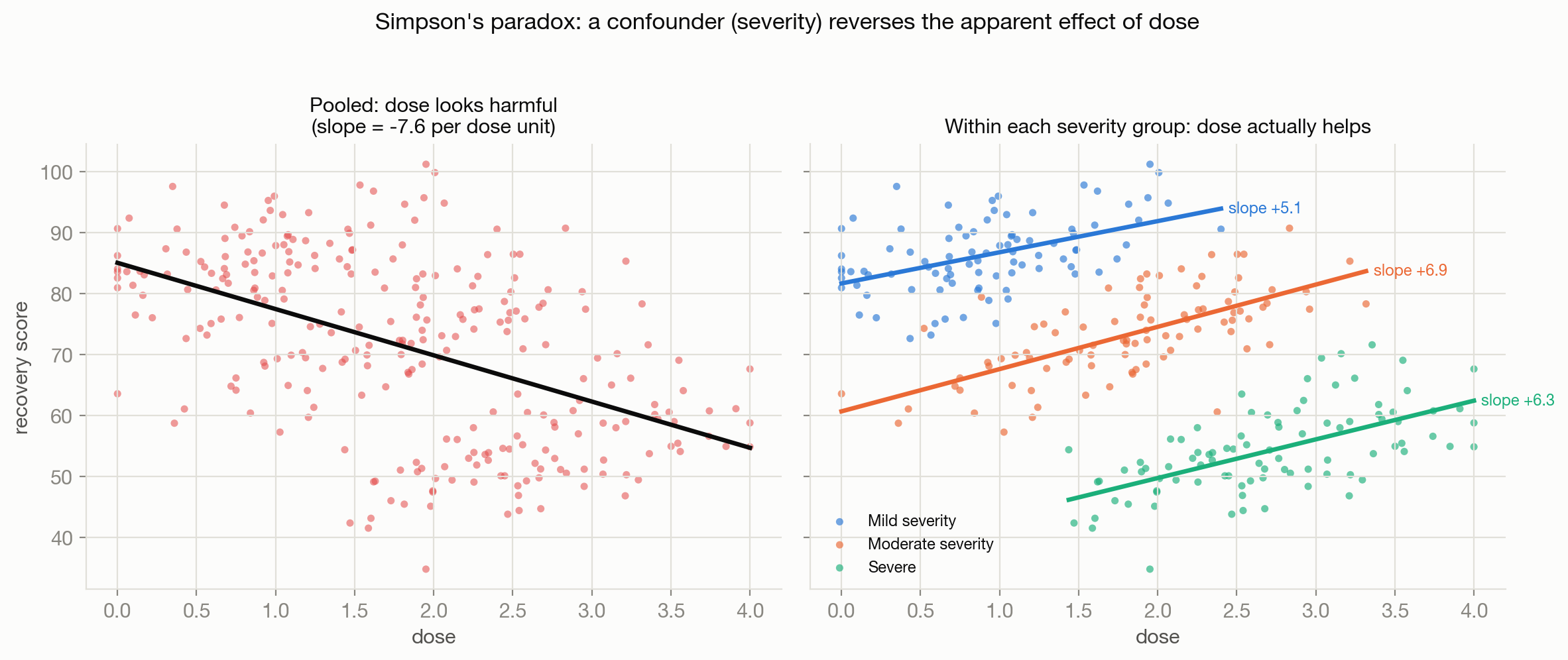
Confounding is what happens when the decision to treat a unit correlates with factors that also affect its outcome. If sicker patients are more likely to receive a stronger dose because their doctors dose up for severe cases, and severity also predicts poor recovery independent of dose, then naively regressing recovery on dose will show a negative association between dose and recovery — even if the drug genuinely helps every single patient. This is Simpson’s paradox: an association that reverses sign once you condition on the right variable. Figure 17.1 shows exactly this, simulated. Pooling across three severity bands, higher-dose patients recover worse on average — a purely confounded, misleading trend, because severity drives both the dose a patient receives and their prognosis. Look within any single severity band, though, and the true effect appears: dose helps recovery in every group. The pooled trend is not “a weaker version of the truth” — it has the opposite sign from the truth. This is the central danger of observational causal claims: the visible correlation and the causal effect can point in different directions, and nothing about the raw data tells you which one you’re looking at.
Causal graphs (directed acyclic graphs, or DAGs) formalize which variables need to be adjusted for and which must not be. A variable is a confounder if it causally affects both treatment and outcome — it must be conditioned on (adjusted for) to block the spurious path. A variable is a collider if both treatment and outcome cause it — conditioning on a collider creates a spurious association where none existed, which is the classic mistake of “controlling for everything available” without checking the graph. A mediator sits on the causal path from treatment to outcome; adjusting for it removes part of the very effect you’re trying to measure. The practical skill in causal inference is almost entirely this: drawing (or at least reasoning through) the assumed causal graph, and choosing an adjustment set that blocks confounding paths without touching mediators or colliders.
Two conditions make a causal estimate identifiable from observational data: unconfoundedness (also called ignorability) — no unmeasured variable affects both treatment assignment and outcome, conditional on the observed covariates — and positivity (overlap) — every unit had a nonzero probability of receiving each treatment level given its covariates. Unconfoundedness is fundamentally untestable from the data at hand, since it is a claim about the absence of unmeasured variables; it can only be argued for on domain grounds or bypassed by design (randomization) or by methods (instrumental variables) that don’t need it.
17.2 Main methods
Randomized experiments
Randomization is the cleanest solution to confounding available: if treatment assignment is decided by a coin flip independent of everything else, then by construction treatment cannot correlate with any confounder, measured or not, and the simple difference in group means is an unbiased estimate of the ATE. This is why A/B testing is the default tool for product causal questions whenever it’s feasible — it sidesteps the entire identification problem that observational methods have to solve with assumptions.
Running a trustworthy experiment is nonetheless its own discipline, because several failure modes can quietly break the “randomization implies validity” guarantee:
- Unit of randomization. Randomizing individual page views when the actual decision-relevant unit is the user (who returns across sessions) contaminates the comparison, since a user can land in both arms over time. The unit of randomization should match the level at which the treatment is meant to have an effect.
- Sample ratio mismatch (SRM). If the traffic split arriving in each arm deviates from the intended ratio (e.g. 50/50 becomes 49/51) by more than chance would explain, something in the randomization or logging pipeline is broken — bot filtering, a redirect bug, differential dropout — and the experiment’s headline result should not be trusted until the mismatch is explained. Checking for SRM with a simple chi-squared test is close to a mandatory first step before reading any other result.
- Interference (SUTVA violations). The stable unit treatment value assumption says one unit’s outcome shouldn’t depend on another unit’s treatment assignment. It’s violated constantly in networked or marketplace settings — a referral feature shown to treated users spills into control users’ feeds, or a treated seller’s discounted price shifts demand away from a control seller in the same market. Interference biases the naive treatment effect estimate, sometimes toward zero (if the spillover pushes control units toward the treated outcome) and sometimes away from it.
- Novelty and primacy effects. A treatment can look effective purely because it’s new and users engage with anything unfamiliar, an effect that decays over the following weeks; the reverse also happens, where users need time to adapt to a change before its true effect shows. Reading an effect estimate from day one of an experiment can be actively misleading in either direction.
- Guardrail metrics. A primary success metric can improve while an unmonitored metric it trades against — latency, revenue, unsubscribe rate — quietly gets worse. Every experiment worth shipping needs guardrails defined in advance, not metrics chosen after the fact to explain away a bad result.
- Multiple testing. Running many metrics or many segment cuts on one experiment inflates the chance that something looks significant by pure chance. Pre-registering the primary metric and correcting explicitly (Bonferroni, false discovery rate control) for any exploratory cuts is what keeps an experimentation platform from becoming a random-result generator at scale.
Observational methods
When randomization isn’t feasible — retrospective medical data, historical pricing changes, policy rollouts that couldn’t ethically or legally be randomized — the identification burden shifts onto assumptions and design.
- Matching. Pair each treated unit with one or more untreated units that look similar on observed covariates, then compare outcomes within pairs. This directly targets unconfoundedness by construction but only along observed dimensions, and it degrades badly in high dimensions since exact matches become rare (the curse of dimensionality).
- Propensity score weighting. Model \(P(\text{treatment} \mid X)\) — the propensity score — and reweight units by the inverse of their propensity to construct a pseudo-population where treatment is balanced across covariates, similar in spirit to importance sampling. This collapses high-dimensional matching into a one-dimensional balancing problem, at the cost of being sensitive to propensity scores near 0 or 1 (a positivity violation), where inverse weights explode.
- Difference-in-differences. Compares the change in outcome over time between a treated group and a control group, rather than a single-period level comparison. This cancels out any time-invariant confounder between groups (the classic use case: a policy rolled out in one state but not a neighboring one), under the assumption that the two groups would have followed parallel trends absent the treatment — a strong, checkable-only via-pre-trends assumption.
- Regression discontinuity. Exploits a hard threshold rule — eligibility cutoffs, credit score thresholds, test-score admission bars — where units just above and just below the cutoff are treated as good local comparisons for each other, since which side of an arbitrary threshold a unit falls on is plausibly as good as random near the boundary. This buys a very credible local causal estimate at the cost of only being informative near the cutoff, not for the whole population.
- Instrumental variables. Finds a variable \(Z\) that affects treatment but has no direct effect on the outcome except through treatment (the exclusion restriction), then uses the variation in treatment driven purely by \(Z\) to estimate the effect — this is the one method on this list that doesn’t require unconfoundedness, but it lives or dies on the exclusion restriction, which is an assumption about the world, not something a dataset can confirm.
- Causal graphs and adjustment sets. Rather than a specific estimator, drawing the assumed DAG and applying the backdoor criterion (formally identifying which adjustment sets block all confounding paths without opening any collider paths) is the general-purpose tool that tells you which of the above methods is even valid for a given question, and what to condition on if you use matching or weighting.
Uplift and policy learning
Sometimes the actionable question isn’t “who is at risk” but “who will respond to an intervention” — this is treatment effect modeling, usually called uplift or CATE (conditional average treatment effect) modeling. The target is \(\tau(x) = \mathbb{E}[Y(1) - Y(0) \mid X = x]\), the treatment effect as a function of covariates, not \(P(Y \mid X)\). A churn prediction model ranks users by risk; a churn prevention policy should rank users by how much an intervention would move their outcome, and these rankings can be almost unrelated. A user with very high churn risk might churn regardless of any discount offered (a “lost cause”), and a user with very low churn risk might have stayed anyway (a “sure thing”) — sending either of them the discount wastes it. The users worth targeting are the “persuadables,” where \(\tau(x)\) is large, and a model that only sees \(P(Y \mid X)\) has no way to distinguish a persuadable user from a lost cause, because both can carry identical predicted risk while having opposite treatment effects. Uplift models are typically built either as two separate outcome models (one per treatment arm, subtracted — the “T-learner”) or as a single model that directly targets the difference (the “X-learner” and related meta-learners), usually trained on data from a randomized experiment so that \(\tau(x)\) is actually identifiable rather than confounded.
17.3 When to use it / what can go wrong
Reach for a randomized experiment whenever the decision is feasible to test live and the population is large enough to power a clean read — it is almost always the most defensible source of a causal claim a business or paper can make. Reach for observational methods when randomization is infeasible, unethical, or too slow, but be explicit and honest about which identification assumption you’re leaning on (unconfoundedness for matching/weighting, parallel trends for diff-in-diff, a valid instrument for IV, local randomness near the cutoff for RDD) — a causal number produced without naming its assumption is not more trustworthy than a correlation, it’s just dressed up as one.
The most common practical failure is treating a prediction model as if it were an intervention-ranking tool. A churn model trained on historical data learns “who looks like the users who churned,” which conflates genuinely at-risk users, users who would have churned regardless of any intervention, and users whose churn risk was itself caused by something correlated with (not affected by) the retention lever available. Deploying it to target an intervention silently assumes that predicted risk and treatment responsiveness are the same thing, which is exactly the assumption uplift modeling exists to avoid making.
Other recurring failure modes worth checking for explicitly: positivity violations (a subgroup that never or always receives treatment in the historical data has no valid comparison and any estimate for it is extrapolation, not inference); interference in networked or marketplace data silently biasing an experiment’s effect size; and multiple testing across dashboards of metrics producing “significant” results that are pure noise. None of these are exotic edge cases — they are the default failure modes of running experimentation and observational analysis at any real scale, and a mature experimentation platform is built explicitly around catching them (SRM checks, guardrail metrics, pre-registered primary metrics, power calculations before launch) rather than trusting a single p-value after the fact.
17.4 How this connects
- Reinforcement Learning and Bandits — bandits and RL are both, at their core, sequential causal inference: choosing actions (interventions) to maximize an outcome, with the exploration/exploitation tradeoff existing precisely because the counterfactual for an untried action is unobserved.
- Information Retrieval, Ranking, and Recommenders — off-policy and counterfactual evaluation of a ranking or recommendation policy from logged data is causal inference applied to logged bandit feedback, using the same propensity-weighting ideas as observational methods here.
- Evaluation and Benchmarking — offline evaluation metrics answer “how good is this model on held-out data,” a prediction question, while online experimentation is what actually answers whether a model change improves outcomes, a causal question — the two are complementary, not substitutes.
- Conformal Prediction — treatment effect estimates need uncertainty quantification too, and conformal methods extend naturally to giving prediction intervals around individual treatment effect estimates, not just outcomes.
- ML Systems and MLOps — running trustworthy experiments at scale (SRM detection, guardrail monitoring, experiment platforms) is itself a production systems problem, not just a statistics problem.